Project 1: Bank Loan Prediction
Introduction
A loan is a thing that is borrowed especially a sum of money, that is expected to be paid back with interest. A bank loan is the most common form of loan capital for an individual or business provided by banks. A borrower has to return the amount with a certain rate of interest over a period of time. Most of the profit for banks comes from loan interest. Loans are the core business of banks. Since most of the income comes from interest, banks have to follow strict rules and regulations for verification of loans because defaults of loans can cost a huge amount of loss to banks. A machine learning model which can accurately predict defaulters can save money and also helps to reduce the approval time. So the main purpose of this project is to make a robust machine learning model to predict the defaulters.
Table of Contents
- Exploratory Data Analysis (EDA)
- Visualizing outliers
- Looking at a unique value in data
- Handling null/missing value
- Handling imbalanced data
- Feature Selection
- Splitting the data for training and testing
- Preprocessing the data for model
- Evaluation Metrics
- Learning Algorithm
- Conclusion
1. Exploratory Data Analysis (EDA)
The very first step to approach any data science/machine learning project should begin by looking at the data. We need to understand what lies inside our data. Understanding the features/attributes is the very first step of the project. We will look at the features of our dataset.
df.columns

Index(['Loan ID', 'Customer ID', 'Loan Status', 'Current Loan Amount', 'Term',
       'Credit Score', 'Annual Income', 'Years in current job',
       'Home Ownership', 'Purpose', 'Monthly Debt', 'Years of Credit History',
       'Months since last delinquent', 'Number of Open Accounts',
       'Number of Credit Problems', 'Current Credit Balance',
       'Maximum Open Credit', 'Bankruptcies', 'Tax Liens'],
      dtype='object')
We have 18 independent features and 1 dependent feature i.e Loan Status in our dataset. The features are self-explanatory.
df.dtypes

Loan ID                          object
Customer ID                      object
Loan Status                      object
Current Loan Amount               int64
Term                             object
Credit Score                    float64
Annual Income                   float64
Years in current job             object
Home Ownership                   object
Purpose                          object
Monthly Debt                    float64
Years of Credit History         float64
Months since last delinquent    float64
Number of Open Accounts           int64
Number of Credit Problems         int64
Current Credit Balance            int64
Maximum Open Credit             float64
Bankruptcies                    float64
Tax Liens                       float64
dtype: object
We can see three types of data types. They are float64, int64, and object.
- int64: It represents the integer features in a dataset.
- float64: It represents the features having numbers with a fractional part, containing one or more decimals.
- object: It represents the features having multiple datatypes including string.
The feature Years in current job is represented as an object which is treated as categorical variable as it contains string and mathematical notation i.e the year is indicated as 8 years or 10+ years but it should be represented as either integer or float. To convert this feature into float we find the string-like years, year, and mathematical notation like ‘+’,'<' and replace with blank space using excel find and replace function.
EDA is an approach to apply different techniques (mostly graphical) to get maximum insight from our data. We can find the descriptive statistics like mean, standard deviation, minimum, maximum, and quartile from the data. We can also see if there are any outliers.
        Current Loan Amount |  Credit Score   |  Annual Income |   Monthly Debt      | Years of Credit History| Months since last delinquent | Number of Open Accounts | Number of Credit Problems | Current Credit Balance | Maximum Open Credit | Bankruptcies     | Tax Liens

count|	1.000000e+05        |	80846.000000  |	8.084600e+04   |	100000.0000  |	100000.000000         |	46859.000000                 |	100000.00000           |	100000.000000      |	1.000000e+05        |	9.999800e+04      |	99796.000000 |	99990.000000
mean |	1.176045e+07        |	1076.456089   |	1.378277e+06   |	18472.412336 |	18.199141             |	34.901321                    | 	11.12853               |	0.168310           |	2.946374e+05        |	7.607984e+05      |	0.117740     |	0.029313
std  |	3.178394e+07        |	1475.403791   |	1.081360e+06   |	12174.992609 |	7.015324              |	21.997829                    |	5.00987                |	0.482705           |	3.761709e+05        |	8.384503e+06      |	0.351424     |	0.258182
min  |	1.080200e+04        |	585.000000    |	7.662700e+04   |	0.000000     |	3.600000              |	0.000000                     |	0.00000                |	0.000000           |	0.000000e+00        |	0.000000e+00      |	0.000000     |	0.000000
25%  |	1.796520e+05        |	705.000000    |	8.488440e+05   |	10214.162500 |	13.500000             |	16.000000                    |	8.00000                |	0.000000           |	1.126700e+05        |	2.734380e+05      |	0.000000     |	0.00000
50%  |	3.122460e+05        |	724.000000    |	1.174162e+06   |	16220.300000 |	16.900000             |	32.000000                    |	10.00000               |	0.000000           |	2.098170e+05        |	4.678740e+05      |	0.000000     |	0.000000
75%  | 	5.249420e+05        |	741.000000    |	1.650663e+06   |	24012.057500 |	21.700000             |	51.000000                    |	14.00000               |	0.000000           |	3.679588e+05        |	7.829580e+05      |	0.000000     |	0.000000
max  |	1.000000e+08        |	7510.000000   |	1.655574e+08   |	435843.280000|	70.500000             |	176.000000                   |	76.00000               |	15.000000          |	3.287897e+07        |	1.539738e+09      |	7.000000     |	15.000000
From the above table, we can find out a data entry/measurement error in credit score. The maximum value of a credit score is 7510 which is impossible. The value of credit score lies within 250-850 or 300-900. So we have to deal with those wrong values (which will be discussed later). The maximum value of the current loan amount is also way too higher than its median which can be a potential outlier in data.
We can also represent our data graphically using histograms and pair plots.
df.hist(bins=50,figsize=(25,10))
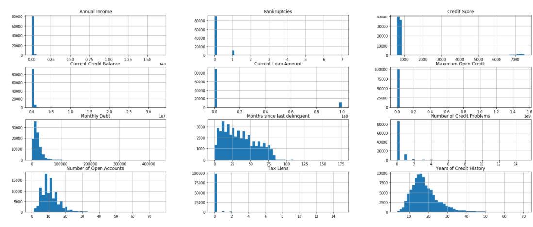
Histograms are graphs that display the distribution of continuous data. Using histograms we can see the distribution and frequency of occurrence of data. We can find the central tendency, variability, skewness, and so on. We can also visualize the outliers using the histogram. In the above figure, we can see that most of the values of credit score are below 1000 but some values are way too far in a graph. Likewise, we can see the same behavior with a current loan amount. The features like years of credit history, a number of open account, months since last delinquent are right-skewed i.e the tail of the distribution extends towards the right.
A pair plot is also very useful while visualizing the single variable or relationship between pair of variables. Pair plot builds on top of the histogram and scatters plot. With seaborn, we can visualize the pair plot. It provides really important insight on which variable separates our classes. But pair plots can’t be useful if we have a large number of features because the number of pair plots becomes very large which makes it difficult to go through all the pair plots. We can use the seaborn library for the pair plot.
sns_plot = sns.pairplot(X,hue='Loan Status')
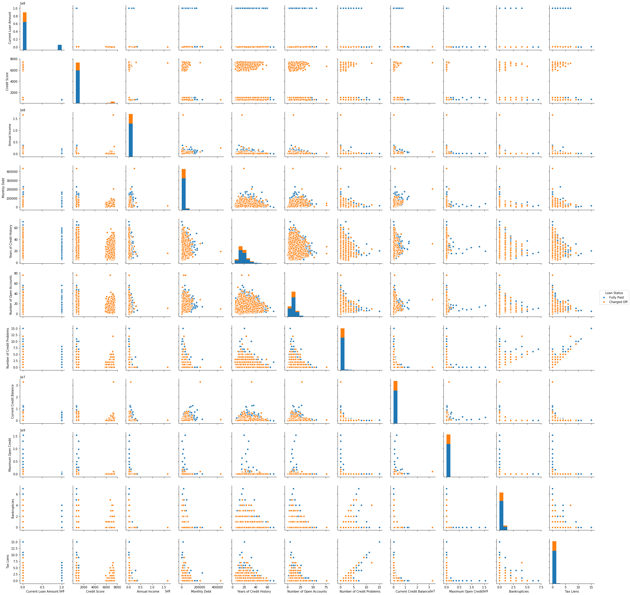
The histogram on the diagonal allows us to visualize the distribution of a single variable while the scatter plots on the upper and lower triangle show the relationship between two variables. We don’t have to look at all plots since the plots in the upper triangle give us the same insight as the lower triangle only the axis is reversed. We see that tax liens and no of credit problem and no of credit problem and bankruptcies are correlated. We also see the classes are well separated. Pair plot also helps to form a simple classification model by drawing some lines or by making the linear separation in our dataset.
2. Visualizing Outliers
Outliers are those data point which is highly deviated from other values in the dataset. Outliers have a high potential to distract our analysis. So, we must take the necessary step to detect and handle the outliers. Visualizing data with help of a boxplot can be helpful to glance at the outliers. Boxplot is based on a five-point summary (minimum, maximum, median, first quartile, and third quartile). There is also a whisker on both sides which ranges up to 1.5 times IQR(difference between first and third quartile) from the upper quartile and 1.5 times IQR below the lower quartile. All the data points which don’t fall within the whisker are considered outliers.
sns.boxplot('Credit Score',data=df)
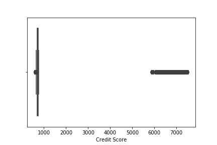
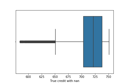
We see lots of outliers in credit scores. As we have discussed earlier, the maximum limit of credit score lies below 900. We have to either remove all the value which contains credit score greater than 900 which will decrease the data point which is not the optimal solution while dealing with outliers or we have to replace the outliers with the mean value of credit score. Carefully looking at the value higher than 900, we can see 0 at the rightmost position of value which seems to have been added accidentally while entering the value. So we will remove 0 from the respective value. Now the boxplot after removing 0.
Similarly, we can also visualize outliers in Current Loan Amount and Maximum Open Credit.
sns.boxplot(x='Loan Status',y='Current Loan Amount',data=df)
sns.boxplot(x='Loan Status',y='Maximum Open Credit',data=df)
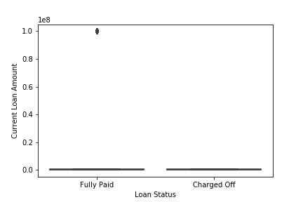
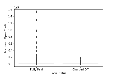
We see that the outliers in Current Loan Amount are present in only a single class Fully Paid i.e who had successfully paid the loan amount while outliers in Maximum Open Credit are also mostly present in Fully paid. The total number of people who have a high Current Loan Amount than it’s mean value is 11484 with Current Loan Amount 99999999.
df_curr = df[df['Current Loan Amount']>df['Current Loan Amount'].mean()]
df_curr['Current Loan Amount'].value_count()

99999999    11484
If we remove those outliers from the dataset then the maximum Current Loan Amount is 789250.
df_curr_less = df[df['Current Loan Amount']<df['Current Loan Amount'].mean()]
df_curr_less['Current Loan Amount'].max()

789250
We see that the outliers are very large as compared to the maximum loan amount without outliers. It might be the case of a data entry error. The digit 9 might have been accidental. Another reason might be of sampling problem. It is because we might accidentally obtain data that are not from the target population. In our case, those data points might come from a businessman. Generally, businessmen borrow more loans from banks to grow their businesses. As the loan is also fully paid, the businessman also pays the loan in time. So, removing those data points mightn’t be the right solution. For such types of problems we can perform analysis without those data points and with those data points then compare the result. But we don’t find other evidence (like businessmen also have high annual income but there is no such information present in their data) to prove that the outlier might be from the sampling problem. So, we will replace those outliers with median values.
3. Looking at the unique value in our data
df_dup = df[df.duplicated()]
df_dup.shape

(10728,19)
10728 rows are duplicated in our dataset which we have to remove. If we look at the unique value in different categorical features we find that the Purpose and Home Ownership feature have a duplicate category.
df['Purpose'].value_counts()
df['Home Ownership'].value_counts()

Debt Consolidation      70834
Home Improvements        5237
other                    5235
Other                    2882
Business Loan            1366
Buy a Car                1165
Medical Bills             983
Buy House                 582
Take a Trip               488
major_purchase            330
small_business            255
moving                    135
wedding                   105
Educational Expenses       91
vacation                   89
renewable_energy            8

Home Mortgage    43548
Rent             37855
Own Home          8199
HaveMortgage       183
We see the other category is duplicated. One begins with a small O and another begins with capital O. So, we can replace those using the excel find and replace option. We will also replace the minority category whose presence is less than 0.5% with other categories.
The Home Ownership feature also has a duplicate category. The two categories Home Mortgage and HaveMortgage represent the same category. We will combine two different categories into a single category i.e Home Mortgage. For this task also we can use the excel find and replace option.
4. Handling null/missing value
We can find the total number of missing values in each feature using pandas function.
df.isna().sum()

Loan ID                             0
Customer ID                         0
Loan Status                         0
Current Loan Amount                 0
Term                                0
Credit Score                    19154
Annual Income                   19154
Years in current job             3802
Home Ownership                      0
Purpose                             0
Monthly Debt                        0
Years of Credit History             0
Months since last delinquent    48337
Number of Open Accounts             0
Number of Credit Problems           0
Current Credit Balance              0
Maximum Open Credit                 2
Bankruptcies                      190
Tax Liens                           9
The percentage of missing value in Months since last delinquent is 48%. Since the percentage of missing value is greater than 30% we will not use this feature in our model. Removing all missing values results in loss of data which we don’t want. We can impute the missing value with mean, median, or mode. We can also try KNN imputation. But here we will use mean, median or mode. If our features are categorical then we use the mode (maximum frequency) to fill missing value. For numerical feature we use mean but if there are outliers then we use median which isn’t sensitive to outliers.
mean = df['Credit Score'].mean()
anninc_mean = df['Annual Income'].mean()
max_open_cre_med = df['Maximum Open Credit'].median()
bank_mode = df['Bankruptcies'].mode()
bank_mode=bank_mode[0]
tax_mode = df['Tax Liens'].mode()
tax_mode=tax_mode[0]
year_cur_mode=df['Years in current job'].mode()
year_cur_mode = year_cur_mode[0]
df['Credit Score'].fillna(value=mean,inplace=True)
df['Bankruptcies'].fillna(value=bank_mode,inplace=True)
df['Tax Liens'].fillna(value=tax_mode,inplace=True)
df['Annual Income'].fillna(value=anninc_mean,inplace=True)
df['Maximum Open Credit'].fillna(value=max_open_cre_med,inplace=True)
df['Years in current job'].fillna(value=year_cur_mode,inplace=True)
5. Handling the imbalanced data
Let’s look at the percentage of each class in dataset.
df['Loan Status'].value_counts(normalize=True)

Fully Paid     0.747853
Charged Off    0.252147
We see that our dataset is not balanced. We need to balance our data otherwise our model will be biased towards the majority class. There are two techniques to handle imbalanced datasets.
- Under Sampling
- Over Sampling
In under-sampling, we reduce the number of data points of the majority class to make the dataset balanced, and in over-sampling, we increase the number of data points of the minority class by duplicating the data points. Most of the time we use oversampling because we don’t want to lose our data. We will use oversampling method to balance the dataset. Duplicating data points to increase data doesn’t add any new information to the model. Instead, new data points are synthesized from the existing data points. This type of method is referred to as Synthetic Minority Oversampling Technique (SMOTE). SMOTE first selects a minority class instance at random and finds its k nearest minority class neighbors. The synthetic instance is then created by choosing one of the k nearest neighbors b at random and connecting a and b to form a line segment in the feature space. The best way of doing SMOTE is not applying SMOTE directly to all data. Once we split our data on train and test then, we only apply SMOTE on train data because all the synthetic data should only be used for training not for validation.
6. Feature Selection
Feature Selection is the process to automatically select those features which contribute most to our model. Having irrelevant features in our data doesn’t increase the accuracy of our model. We want to remove those features which don’t have a significant effect. We can use seaborn library to plot a heat map to study the correlation between features.
df_corr = df[['Current Loan Amount','Credit Score','Years in current job','Annual Income','Monthly Debt','Years of Credit History','Months since last delinquent','Number of Open Accounts','Number of Credit Problems','Current Credit Balance','Maximum Open Credit','Bankruptcies','Tax Liens']]
plt.figure(figsize=(12,12))
sns.heatmap(df_corr.corr(),annot=True,cmap='coolwarm')
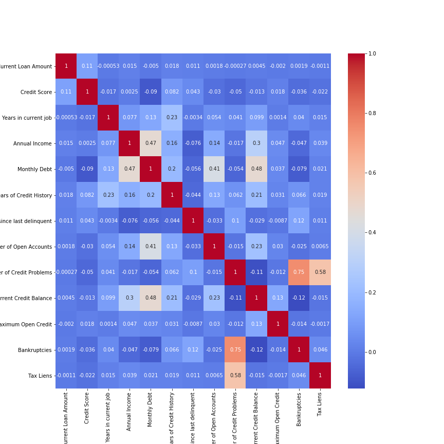
We see our most of the features are not highly correlated with each other. Two features Number of Credit Problems and Bankruptcies are correlated with each other. Instead, if two features are perfectly correlated, then one doesn’t add any additional information. So removing either of the features doesn’t affect the accuracy of the model. We can also use the Variance Inflation Factor (VIF) for feature selection. VIF is the measure of the amount of multicollinearity in a set of features. We can find the VIF of the respective feature and remove the feature having VIF greater than 10. VIF is calculated by keeping one independent variable as dependent and another independent variable as it is and fitting a linear regression model to calculate the coefficient of determination. The coefficient of determination represents the total variation for a dependent variable that is explained by independent variables. After calculating the coefficient of determination we can find VIF by using the formula.
df_vif = df[['Current Loan Amount','Credit Score','Years in current job','Annual Income','Monthly Debt','Years of Credit History','Number of Open Accounts','Number of Credit Problems','Current Credit Balance','Maximum Open Credit','Bankruptcies','Tax Liens']]
vif = [variance_inflation_factor(df_vif.values, i) for i in range(df_vif.shape[1])]
for i in range(0,len(vif)):
    print("The vif for {} is {}".format(df_vif.columns[i],vif[i]))
The vif for Current Loan Amount is 5.216088749985775
The vif for Credit Score is 14.133526238670429
The vif for Years in current job is 4.285574183873071
The vif for Annual Income is 3.8662576896476977
The vif for Monthly Debt is 5.9926280268315
The vif for Years of Credit History is 8.723717621178784
The vif for Number of Open Accounts is 7.196910622526113
The vif for Number of Credit Problems is 8.399897979508326
The vif for Current Credit Balance is 2.253278721025104
The vif for Maximum Open Credit is 1.0296436972885672
The vif for Bankruptcies is 5.516843092735326
The vif for Tax Liens is 3.2920982116858917
We see the VIF for Credit Score is greater than 10 so we will remove this feature from the dataset. Removing those features having high VIF doesn’t affect our accuracy or prediction but it is better to remove those variables which don’t add value to our model.
7. Splitting the data
Now we will split our data into training and testing sets. This allows us to validate our model on unseen data. We will use stratified train_test_split as the number of classes is highly imbalanced. It preserves the percentage of samples from each class.
X = df[['Current Loan Amount', 'Term', 'Annual Income', 'Years in current job', 'Home Ownership', 'Purpose', 'Monthly Debt', 'Years of Credit History', 'Number of Open Accounts','Number of Credit Problems', 'Current Credit Balance','Maximum Open Credit', 'Bankruptcies', 'Tax Liens']]
Y = df['Loan Status']
X_train,X_test,y_train,y_test = train_test_split(X,Y,test_size=0.2 ,random_state=42,stratify=df['Loan Status'])
8. Preprocessing the data
First of all, we will remove the unnecessary features like Loan ID and Customer ID which are the unique values assigned to each customer. Those features don’t add any information to our model. Before feeding our data into model we need to encode the categorical value into numerical value. Categorical value refers to the information that has specific categories within the dataset. There are four categorical features in our dataset i.e Loan Status, Term, Home Ownership, Purpose. We can use LabelEncode() class from sci-kit learn library to encode the categorical value. The code will be as follows:
labelencoder = LabelEncoder()
df.iloc[:,2] = labelencoder.fit_transform(df.iloc[:,2])
df.iloc[:,4] = labelencoder.fit_transform(df.iloc[:,4])
df.iloc[:,8] = labelencoder.fit_transform(df.iloc[:,8])
df.iloc[:,9] = labelencoder.fit_transform(df.iloc[:,9])
Label encoding has the disadvantage that the numeric value can be misinterpreted by some of the algorithms as having order to them. The string will be assigned numbers in increasing alphabetical order. The machine learning model captures the relationship between the categories based on those orders which are not preferred. Instead, we use a different technique for treating categorical variables i.e One Hot Encoding. One Hot Encoding creates an additional feature based on the number of unique values in the features. Then every unique value will be treated as a feature consisting of binary data either 0 or 1.
df = pd.get_dummies(df,columns=['Home Ownership','Purpose'])
Tree-based models don’t perform well with one hot encoding if there are too many unique values in the feature. This is because they pick the subset of the feature while splitting the data. If we have a lot of unique value, then the chosen features will be mostly zero which doesn’t produce a significant result. So we don’t perform one hot encoding while training tree-based models. Linear models don’t suffer from this problem.
The next step for preprocessing is scaling the features. There are various methods to scale the data like standardization, min-max scaler, etc. In the min-max scaler, we simply subtract the minimum value of the feature from the current value and divide it by the difference of maximum and minimum value. This technique re-scales a feature value between 0 and 1. In standardization, we subtract the mean from the current value and divide it by standard deviation. Standardization re-scales a feature value having mean 0 and variance 1. Feature scaling is important when there is a large difference in the magnitude of different features. Generally, tree-based models such as random forest, decision tree doesn’t require feature scaling but the distance-based model and neural network are highly affected by scaling.
std = StandardScaler()
X_train_sc = std.fit_transform(X_train)
X_test_sc = std.transform(X_test)
9. Evaluation Metrics
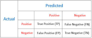
Evaluation metrics are used to measure the performance of the machine learning model. For classification problem, accuracy is the most frequently used evaluation metrics. However, it is not always true and can be misleading when our data is imbalanced. Evaluation of the performance of a classification model is based on the counts of test records correctly and incorrectly predicted by the model. The confusion matrix is often used to describe the performance of the classification model. We can calculate accuracy, recall, precision, and f1 score from the confusion matrix. The confusion matrix for binary classification consists of true positive, true negative, false positive, false negative.
-
True Positive: These are cases in which we predicted positive i.e. those who will repay the loan and they have paid the loan.
-
True Negative: These are cases in which we predicted negative i.e. those who will default and they have defaulted.
-
False Positive: These are cases in which we predicted positive but they defaulted.
-
False Negative: These are cases in which we predicted negative but they paid the loan.
In our case, we care about those predictions which are false-positive which is when it predicts positive how often is it correct. We want to minimize the number of false positives. Instead, we care about high precision.
10. Learning Algorithm
Choosing the right algorithm is also an important phase of a data science project. Since our project is a classification problem we can choose a variety of classification algorithms to make a prediction. Some of the algorithms we have used are listed below:
- Logistic Regression
- K Nearest Neighbors
- Support Vector Machine
- Random Forest Classifier
-
Logistic Regression:
Logistic regression is one of the classical classification methods. It is the most commonly used algorithm for solving a classification problem. Logistic regression can be used for binary classification i.e. when the target variable has two classes and multinomial classification i.e. when the target variable has more than two classes. Logistic regression is named for the function used “logistic function”. The logistic function is also called the sigmoid function. The logistic function gives an “S” shape curve that can take any real value and map it into a value between 0 and 1. If the output of the function is greater than 0.5, we classify the output as 1 and if the output is less than 0.5, we classify the output as 0. Below is the figure of the sigmoid function.
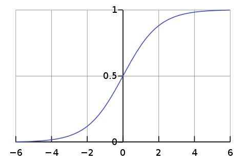
Image Source: From Wikipedia
We will use sklearn library to implement logistic regression. Since our data set is imbalanced evaluating our model based on accuracy gives us misleading results. We use a confusion matrix to show the correct and incorrect predictions. We want to decrease the false positive while maintaining acceptable false negative. We will use a different value of the upsampling ratio for training and compare their result.
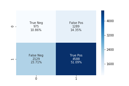
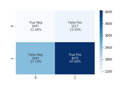
The accuracy using the upsampling ratio of 0.8 is 69% and the confusion matrix is shown in the below figure.
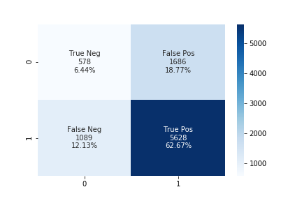
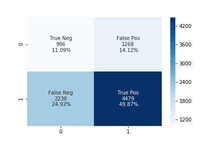
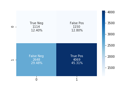
The accuracy using the upsampling ratio of 0.9 is 61% and the confusion matrix is shown in the below figure.
The accuracy using the upsampling ratio of 1.0 is 54% and the confusion matrix is shown in the below figure.
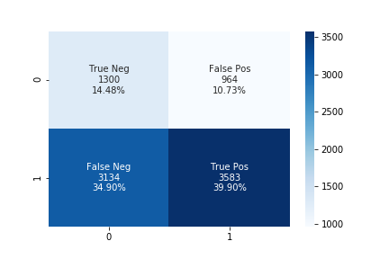
We can see that while increasing the upsampling ratio the accuracy of the model decrease. The number of false-positive also decreases while increasing the upsampling ratio at the same time the number of false-negative also increases. In such a case, we can use some threshold values for false-negative and choose the best-performing model according to our needs.
-
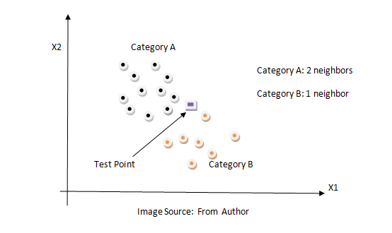
K Nearest Neighbors:
KNN is a non-parametric classification method. It is used for classification and regression problems. It is one of the simplest algorithms. The key idea of the KNN algorithm is nearby points belong to the same class. KNN algorithm makes no assumption about the data. It computes the distance between the testing point to every training example. Then select the k closest instances and their labels. It output the class which is most frequent in labels. The training time of the KNN algorithm is zero while the testing time can become very large with a large number of data points in the dataset. This algorithm can be computationally expensive because we need to store all training examples and compute the distance to all training examples for a single prediction. Below is the figure of how the KNN algorithm works.
We can use the same method described above.
The accuracy using the upsampling ratio of 0.8 is 61% and the confusion matrix is shown in the below figure.
The accuracy using the upsampling ratio of 0.9 is 59% and the confusion matrix is shown in the below figure.
The accuracy using the upsampling ratio of 1.0 is 57% and the confusion matrix is shown in the below figure.
-
Support Vector Machine:
Support Vector Machine is a supervised learning model that analyzes data for classification and regression analysis. It constructs a hyperplane in high dimension space which can be used for classification or regression. It finds a hyperplane that has the largest distance to the nearest training data points. The closest points are called support vectors and hence algorithm is termed a Support Vector Machine. The distance from the nearest training point to the hyperplane is called margin. It tries to maximize the margin. So SVM is also called a max-margin classifier. Max margin can reduce the effect of mislabelled data than min margin and it generalizes better in the future for unseen data. SVM is effective in high dimensional space because data are likely to be linearly separable in high dimensions than in low dimensions. Below is the figure SVM algorithm.
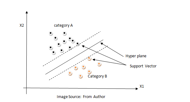
We tried the different values of upsampling ratio but the results were the same. The accuracy of the linear SVM model is 73% and the confusion matrix is shown in the below figure.

-
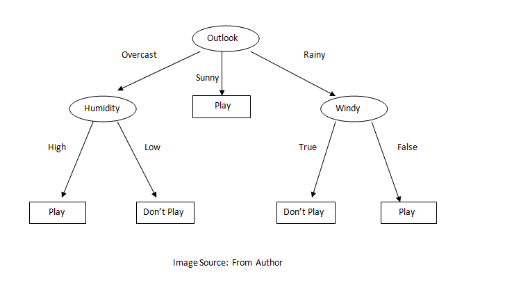
Random Forest Classifier:
Random Forest is an ensemble learning method for classification and regression problems. A random forest fits several decision trees on various sub-sample of the dataset and outputs the class that is a mode of the classes for classification problem and mean/average of the individual tree for a regression problem. A decision tree is a very powerful and intuitive model. The idea of the decision tree is to divide the space into different regions and fit a very simple model to each region. The model can be linear or constant. To divide into different spaces we use the simple if-else rule that provides branching. We need to select the best attribute/features to generate the branching. To select the attribute at the root we can use some criterion like information gain, Gini index, etc. In the case of information gain, we find the gain of all attributes and attribute with the highest gain is placed at the root, and branches with entropy greater than 0 needs further splitting. In this way, we can create a decision tree. Decision trees suffer from overfitting but random forest controls the problem of overfitting. In a random forest, features and datapoint are randomly chosen so that the tree is independent of each other as a result it reduces the high variance problem of the decision tree. Below is the figure of the decision tree.
We can use the same method described above.
The accuracy using the upsampling ratio of 0.8 is 71% and the confusion matrix is shown in the below figure.

The accuracy using the upsampling ratio of 0.9 is 70% and the confusion matrix is shown in the below figure.

The accuracy using the upsampling ratio of 1.0 is 70% and the confusion matrix is shown in the below figure.

Analyzing the above confusion matrix, we can see the performance of different algorithms varies significantly. SVM doesn’t perform well as it is predicting only a single class for all of the data. At the upsampling ratio of 1.0 logistic regression has the lowest number of false positives as compared to another algorithm which is also the desired objective of our problem. The decrease in false-positive came at the cost of the increase in false negatives.
The plot below shows the number of true positive, true negative, false positive, false negative for different values of n_neighbor and n_estimator in KNN and Random Forest algorithm respectively.
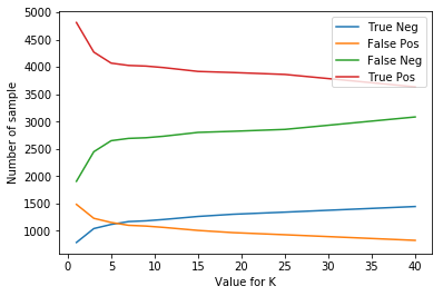
Total number of TP TN FP FN for different value of neighbors in KNN
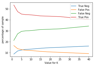
Total percentage of TP TN FP FN for different value of neighbors in KNN
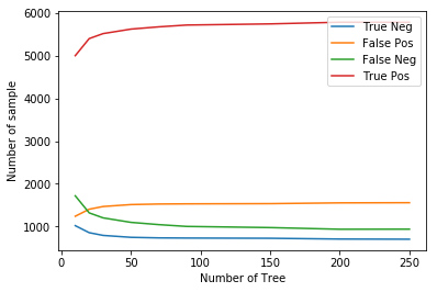
Total number of TP TN FP FN for different value of n_estimators in Random Forest
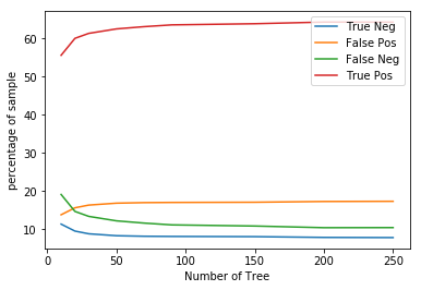
Total percentage of TP TN FP FN for different value of n_estimators in Random Forest
From the above plot, we see that if we increase the neighbors in the KNN algorithm then the false positive decrease while the false negative increase and if we decrease the neighbors then false positive increases while false negative decreases. In Random Forest, if we increase the number of the tree then false positive increase while false negative decrease, and if we decrease the number of the tree the false-positive decrease while false negative increase. In such cases, we can select a model according to the need of our project.
11. Conclusion
In this article “Bank Loan Prediction”, we discussed the pipeline of a data science/machine learning project. Finally, we achieved the goal of this project i.e to correctly predict defaulters with the help of different machine learning algorithms. We hope such a system can be deployed in real-world situations after further refinement which can be very useful and interesting for the banking sector.
12. Links
The code for the project can be found Here
The original dataset can be found Here